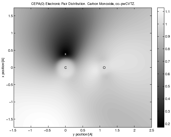
The following script produces this picture (as eps, it is a contour plot, for more information on what this is, see the comment at the start of the script):

The script calculates a so called two-particle reduced density matrix (for CEPA(0)) and then uses this one to calculate the electronic pair-density and pair-distribution functions for a given reference point.
"""This script makes pictures of CEPA(0) electronic pair distribution functions:
                    <\Psi^+(r) \Psi^+(r') \Psi(r')  \Psi^(r)>
        g(r,r') =   ------------------------------------------- .
                    <\Psi^+(r) \Psi^(r)> <\Psi^+(r') \Psi(r')>

these functions directly show the so called electronic correlation hole, i.e.
they visualize how electrons avoid each other: g(r,r') is the probability
of finding an electron at place r' PROVIDED one _has_ already been found
at place r (divided by the independent probabilities).
The Hartree-Fock deficiency, i.e. the reason why it often doesn't produce
quantitatively correct results for e.g. binding energies or some observables,
is precisely that HF does not predict this function correctly.

This script now calculates such functions for the correlated CEPA(0) theory
by fixing one of the points (r) and tabulating the values of g(r,r') on a grid.
Then a matlab script is generated which turns the grid data into a picture.

Note: The calculating of the two-particle reduced density matrix, which is
required in order to perform this calculation, requires A LOT OF RAM. A
direct integrator won't help.
"""

from ct8k import *
from ct8kpy import *

import os

SetOutputUnits( ENERGY_Hartree, DISTANCE_Angstrom )
MainDir = "../"

for Basis in ["cc-pVDZ","cc-pVTZ","aug-cc-pVDZ","aug-cc-pVTZ",
    "cc-pwCVDZ","cc-pwCVTZ","PairDensityX"]:

    LoadBasisLibrary( MainDir + "basis_lib/%s.libmol" % Basis )

RefPoints = []
FileSuffices = []


File = MainDir + "molecules/co_yx.xyz"

MoleculeName = "CO"
MoleculeFull = "Carbon Monoxide"
Basis = "cc-pwCVTZ"

# range (in angstroem) of the plot region
(MinX, MaxX, MinY, MaxY ) = ( -1.5, +2.5, -2.0/1.15, +2.0/1.15 )

# resolution of the density grid. And range in distance units
# covered.
(GridResX,GridResY) = (140,140)
TransposeXy = True

RefPoints += [FVector3( 0.0, 0.4, 0.0 )]

FileSuffices += [""]


def main():

    DistUnitFactor = ConvertDistance(1.0)

    for (RefPoint, FileSuffix) in zip( RefPoints, FileSuffices ):

        # we need to specify the basis position in atomic units.
        RefPointAu = FVector3( RefPoint.get(0)/DistUnitFactor,

            RefPoint.get(1)/DistUnitFactor, RefPoint.get(2)/DistUnitFactor )

        # load atoms and add some more basis functions at the reference point
        Atoms = FAtomSet()
        Atoms.AddAtomsFromXyzFile( File, Basis )

        Atoms.AddAtom( FAtom( RefPointAu, "XX", "PAIRX" ) )

        # perform a HF and a CEPA calculation. If we would not add the
        # additional basis functions at the ref point, we would actually
        # need to do that only once, not once per ref point.
        (Converged, Energy, HfResult, HfParams) = \
            HartreeFock( Atoms, DensityThreshold = 1e-7, MinIterations = 15 );

        assert( Converged )

        # drop the Integrator in order to free the memory associated with it.
        (Converged, Energy, CepaResult) = \
            Cepa( HfResult, HfParams.pIntegrator,

            Method = METHOD_Cepa0, NumCoreOrbitals = 0, Want1Rdm = True,

            Want2Rdm = True, ResidualThreshold = 1e-5 );

        # drop the Integrator in order to free the memory associated with it.
        HfParams.SetIntegrator(None)

        Z = 0.0

        # make a 2D grid on which the pair density will be calculated.
        # Params: ResX, ResY, x-Increment, y-Increment, GridOrigin.
        DensityGrid = FScalarGrid( GridResX, GridResY,

            FVector3( (MaxX - MinX)/( GridResX - 1 )/DistUnitFactor, 0.0, 0.0 ),

            FVector3( 0.0, (MaxY - MinY)/( GridResY - 1 )/DistUnitFactor, 0.0 ),

            FVector3( MinX/DistUnitFactor, MinY/DistUnitFactor,
                        Z/DistUnitFactor ) );


        print "calculating density on grid..."
        #MakeDensityGrid( DensityGrid,CisdResult.DensityAO,HfParams.pBasisSet );
        MakePairDistributionGrid( DensityGrid,
            RefPointAu, CepaResult.DensityAO, CepaResult.PairDensityEvalContext,

            HfResult.OrbitalSet.Orbitals, HfParams.pBasisSet )
        del CepaResult

        # write out a file containing the data points we produced
        TargetDir = MainDir + "results/"
        DGridFileMain = "pgrid_py_%s%s_%s" % ( MoleculeName, FileSuffix,

                Basis.replace('-','_') )
        DGridFile = TargetDir + DGridFileMain + ".dat"

        DensityGrid.WriteFile( DGridFile );

        # get atom coords in order to make labels on the atoms in the matlab
        # picture.
        AtomCoords = AtomCoordsFromXyzFile(File)

        AtomCoords += [('x', RefPoint.get(0), RefPoint.get(1), RefPoint.get(2))]

        def MakeMatlabFigCommands():
            AtomLabels = ""
            for Atom in AtomCoords:

                AtomLabels += ("text(%g,%g,'%s','Color','%s','horizontalAlig" +\
                    "nment','center','verticalAlignment','middle');\n") \
                    % ( Atom[1], Atom[2], Atom[0], ["k","w"][Atom[0] == "x"] )

            DensityMin, DensityMax, DensityStep = (-4.0, 4.0, 0.01 )

            #DensityScale = 1.0/(DistUnitFactor**3)
            DensityScale = 1.0
            Title = "CEPA(0) Electronic Pair Distribution. %s, %s." \
                    % ( MoleculeFull, Basis )


            # the string produced here will be %'ed with
            # (DensityMin, DensityStep, DensityMax)
            DrawCommand = "" +\
                ";\n" +\
                "'%g';\n" +\
                "[C,h] = contourf(X,Y,pgrid," +\
                    "min(min(pgrid)):%g:max(max(pgrid)),':');\n" +\
                "'%g'\n" +\
                "linc = linspace(0.0,1.0,255);\n" +\
                "ColorGrad = linc;\n"+\
                "InvGray = transpose([ColorGrad;ColorGrad;ColorGrad]);\n"+\
                "colormap(InvGray);\n"+\
                "colorbar();\n" +\
                "set(h,'LineStyle','none');\n" +\
                "\n" +\
                "%% hold on; [C2,h2] = contour(X,Y,pgrid,0:0.05:1);\n" +\
                "%% set(h2,'LineStyle',':'); set(h2,'LineColor',[0,0,0]);\n" +\
                "%% clabel(C2,h2,'Color',[0,0,0]);\n"

            return \
                ( "load %s\n" +\
                "pgrid=%g*%s\n" +\
                "X = linspace(%g,%g,size(pgrid,2))\n" +\
                "Y = linspace(%g,%g,size(pgrid,1))\n" +\
                "%s\n"+\
                "xlabel('%s position/[A]'); ylabel('%s position/[A]' )\n" +\
                "%s\n" +\
                "\n" +\
                "title('%s')\n" +\
                "print('-depsc', '%s')\n" ) \
                % ( DGridFile, DensityScale, DGridFileMain, MinX,MaxX,MinY,MaxY,

                    DrawCommand % ( DensityMin, DensityStep, DensityMax ),

                    ["x","y"][TransposeXy], ["y","x"][TransposeXy],

                    AtomLabels, Title, TargetDir + DGridFileMain )

        MatlabFileName = TargetDir + DGridFileMain + ".m.txt"

        MatlabFile = open( MatlabFileName, 'w' )
        MatlabFile.write( MakeMatlabFigCommands() )

        MatlabFile.close()
        print "calling matlab..."
        os.system("matlab < %s" % MatlabFileName )

main()