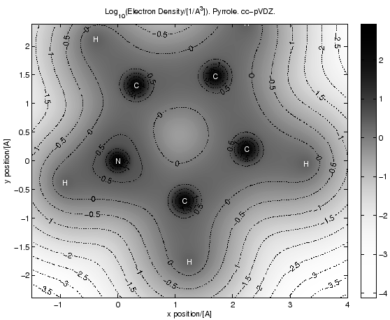
The following script produces this picture (as eps, it is a contour plot):
In this case the script does a CISD correlation calculation and then uses the CISD density matrix to evaluate the electron density on a grid. It then goes on to create a Matlab-script which draws the picture (a much cleaner version of most of this script is in the Correlation Hole example, you should look at that first).
"""This script makes pictures of Hartree-Fock or CISD electron density
distributions on a grid. It does that by first performing a correlation
calculation and then extracting the electron densities out of the density
matrix. It then generates and executes a matlab script which makes
the pictures. (should be ported to matplotlib, a python-interfaced
free matlab clone. Don't have time to do that however) (cgk)"""

from ct8k import *
from ct8kpy import *
import os

SetOutputUnits( ENERGY_Hartree, DISTANCE_Angstrom )
MainDir = "../"
for Basis in ["cc-pVDZ","cc-pVTZ","aug-cc-pVDZ","aug-cc-pVTZ"]:
    LoadBasisLibrary( MainDir + "basis_lib/%s.libmol" % Basis )

DRAWMODE_Density, DRAWMODE_DensityDiff, DRAWMODE_RelDensityDiff = range(3)

File = MainDir + "molecules/pyrrole.xyz"
MoleculeName = "pyrrole"
MoleculeFull = "Pyrrole"
Basis = "cc-pVDZ"
# range (in angstroem) of the plot region
(MinX, MaxX, MinY, MaxY ) = ( -1.5, +4.0, -2.75/1.15, +2.75/1.15 )
# resolution of the density grid. And range in distance units
# covered.
(GridResX,GridResY) = (140,140)
TransposeXy = False
DrawMode = DRAWMODE_Density


def main():
    Atoms = FAtomSet()
    Atoms.AddAtomsFromXyzFile( File, Basis )

    (Converged, Energy, HfResult, HfParams) = \
        HartreeFock( Atoms, DensityThreshold = 1e-7 );
    assert( Converged )

    (Converged, Energy, CisdResult) = \
        Cepa( HfResult, HfParams.pIntegrator,
        Method = METHOD_Cisd, Want1Rdm = True,
        NumCoreOrbitals = 0, ResidualThreshold = 1e-5 );
    #   ResidualThreshold = 1e-4 )

    Z = 0.0
    DistUnitFactor = ConvertDistance(1.0)
    print "Distance Unit Factor: ", DistUnitFactor

    DensityGrid = FScalarGrid( GridResX, GridResY,
        FVector3( (MaxX - MinX)/( GridResX - 1 )/DistUnitFactor, 0.0, 0.0 ),
        FVector3( 0.0, (MaxY - MinY)/( GridResY - 1 )/DistUnitFactor, 0.0 ),
        FVector3( MinX/DistUnitFactor, MinY/DistUnitFactor, Z/DistUnitFactor ) );

#   print "\nCalculating HF electron density on grid..."
#   MakeDensityGrid( DensityGrid, HfResult.ChargeDensityAO, HfParams.pBasisSet );
    if ( DrawMode == DRAWMODE_Density ):
        print "\nCalculating CISD electron density on grid..."
        MakeDensityGrid( DensityGrid, CisdResult.DensityAO, HfParams.pBasisSet );
    else:
        print "\nCalculating CISD - HF difference density on grid..."
        CisdResult.DensityAO -= HfResult.ChargeDensityAO
        MakeDensityGrid( DensityGrid, CisdResult.DensityAO,
            HfParams.pBasisSet );

    DGridFiles = map( lambda x: x + "_py_%s_%s" % \
        (MoleculeName, Basis.replace('-','_')), ["dgrid","ddiff","ddiffrel"] )
    DGridFileMain = DGridFiles[DrawMode]
    TargetDir = MainDir + "results/"
    DGridFile = TargetDir + DGridFileMain + ".dat"
    DensityGrid.WriteFile( DGridFile );

    AtomCoords = AtomCoordsFromXyzFile(File)

    def MakeMatlabFigCommands():
        AtomLabels = ""
        for Atom in AtomCoords:
            AtomLabels += "text(%g,%g,'%s','Color','w','horizontalAlignment','center','verticalAlignment','middle');\n"  \
                % ( Atom[1], Atom[2], Atom[0] )
        DensityMin, DensityMax, DensityStep = (-4.0, 4.0, [0.03,0.003,0.05][DrawMode] )
        DensityScale = 1.0/(DistUnitFactor**3)
        Title = ["Log_{10}(Electron Density/[1/A^3]). %s. %s.",
                 "Density Difference (n_{CISD}-n_{HF})/[1/A^3]). %s. %s.",
                 "Relative Density Difference 100%%*(n_{CISD}-n_{HF})/n_{CISD}. %s. %s."\
                 ][DrawMode] % ( MoleculeFull, Basis )


        def MakeDrawCommand():
            # the string produced here will be %'ed with
            # (DensityMin, DensityStep, DensityMax)
            if ( DRAWMODE_Density == DrawMode ):
                # drawing total densities. Do this in a logarithmic plot, but
                # adjust the color axis a bit so that it won't just look
                # like everywhere is the same density.
                return "" +\
                    "pgrid = log10(pgrid);\n" +\
                    "'%g';\n" +\
                    "[C,h] = contourf(X,Y,pgrid,min(min(pgrid)):%g:max(max(pgrid)),':');\n" +\
                    "'%g'\n" +\
                    "linc = linspace(0.0,1.0,255);\n" +\
                    "ColorGrad = 1-linc.^(3*(1-linc));\n"+\
                    "InvGray = transpose([ColorGrad;ColorGrad;ColorGrad]);\n"+\
                    "colormap(InvGray);\n"+\
                    "colorbar();\n" +\
                    "set(h,'LineStyle','none');\n" +\
                    "\n" +\
                    "hold on; [C2,h2] = contour(X,Y,pgrid,-5:0.5:2);\n" +\
                    "set(h2,'LineStyle',':'); set(h2,'LineColor',[0,0,0]);\n" +\
                    "clabel(C2,h2,'Color',[0,0,0]);\n"
            elif ( DRAWMODE_DensityDiff == DrawMode ):
                # drawing a density difference. Do this in a linear plot.
                return "" +\
                    "'%g';\n" +\
                    "[C,h] = contourf(X,Y,pgrid,min(min(pgrid)):%g:max(max(pgrid)),':');\n" +\
                    "'%g'\n" +\
                    "linc = linspace(0.0,1.0,1255);\n" +\
                    "ColorGrad = linc.^2.45;\n"+\
                    "ColorGrad = interp1([0,0.25,0.5,0.75,0.85,1.0],[0.0,0.15,0.35,0.5,0.92,1.0],linc,'pchip');\n"+\
                    "InvGray = transpose([ColorGrad;ColorGrad;ColorGrad]);\n"+\
                    "colormap(InvGray);\n"+\
                    "colorbar();\n" +\
                    "set(h,'LineStyle','none');\n" +\
                    "hold on; [C2,h2] = contour(X,Y,pgrid,[0.0,0.1]);\n" +\
                    "set(h2,'LineStyle',':'); set(h2,'LineColor',[0,0,0]);\n" +\
                    "clabel(C2,h2,'Color',[0,0,0]);\n" +\
                    ""
            else: # ( DRAWMODE_DensityDiffRes == DrawMode == 2 )
                return ( "load %(den_f)s; load %(ddif_f)s;\n" +\
                    "pgrid = 100.0 * %(ddif)s ./ %(den)s ;\n" ) % \
                        { "den_f" : TargetDir + DGridFiles[0] + ".dat",
                          "ddif_f" : TargetDir + DGridFiles[2] + ".dat",
                          "den": DGridFiles[0], "ddif": DGridFiles[2] } +\
                    "'%g';\n" +\
                    "[C,h] = contourf(X,Y,pgrid,min(min(pgrid)):%g:max(max(pgrid)),':');\n" +\
                    "'%g'\n" +\
                    "linc = linspace(0.0,1.0,1255);\n" +\
                    "%% ColorGrad = 1 - linc.^0.75;\n"+\
                    "ColorGrad = 1-linc.^(2*(1-linc));\n"+\
                    "InvGray = transpose([ColorGrad;ColorGrad;ColorGrad]);\n"+\
                    "colormap(InvGray);\n" +\
                    "tickrange = [-20:1:20];\n" +\
                    "ticklabels = strcat(cellstr(num2str(transpose(tickrange))),'%%');\n" +\
                    "colorbar('YTick',tickrange,'YTickLabel',ticklabels);\n" +\
                    "set(h,'LineStyle','none');\n" +\
                    "hold on; [C2,h2] = contour(X,Y,pgrid,-10:1:10);\n" +\
                    "set(h2,'LineStyle',':'); set(h2,'LineColor',[0,0,0]);\n" +\
                    "clabel(C2,h2,'Color',[0,0,0]);\n" +\
                    ""

        DrawCommand = MakeDrawCommand()

        return \
            ( "load %s\n" +\
            "pgrid=%g*%s\n" +\
            "X = linspace(%g,%g,size(pgrid,2))\n" +\
            "Y = linspace(%g,%g,size(pgrid,1))\n" +\
            "%s\n"+\
            "xlabel('%s position/[A]'); ylabel('%s position/[A]' )\n" +\
            "%s\n" +\
            "\n" +\
            "title('%s')\n" +\
            "print('-depsc', '%s')\n" ) \
            % ( DGridFile, DensityScale, DGridFileMain, MinX, MaxX, MinY, MaxY,
                DrawCommand % ( DensityMin, DensityStep, DensityMax ),
                ["x","y"][TransposeXy], ["y","x"][TransposeXy],
                AtomLabels, Title, TargetDir + DGridFileMain )
#           "fig = contourf(X,Y,pgrid,%g:%g:%g,':');\n" +\
#           "fig = contourf(X,Y,pgrid,min(min(pgrid)):0.01:max(max(pgrid)),':');\n" +\
#           "c = findobj('LineStyle',':')'; set(c,'LineStyle','none');\n" +\
#           "ColorGrad = 1-((1-linspace(1.0,0.0,255)).^1.5);"+\

    MatlabFileName = TargetDir + DGridFileMain + ".m.txt"
    MatlabFile = open( MatlabFileName, 'w' )
    MatlabFile.write( MakeMatlabFigCommands() )
    MatlabFile.close()
    print "calling matlab..."
    os.system("matlab < %s" % MatlabFileName )

main()